How much spreading comes from the grid?
29 September 2026 · Controlled transport benchmark · AI-assisted research
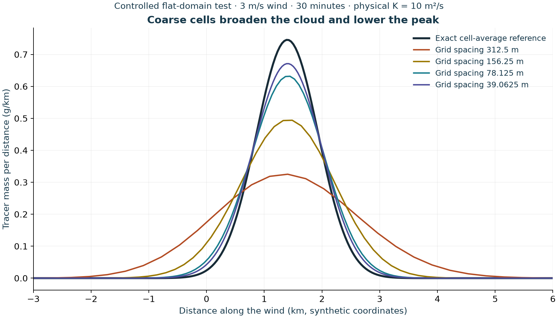
The Explorer's transport method spreads a smooth test cloud too widely at coarse resolution. In a flat, uniform-wind test using the same 312.5 m horizontal spacing as the public map, its peak cell-average concentration is only 44% of the exact reference when physical mixing is set to 10 m²/s. Refining to 39.0625 m raises the peak to 90% of the reference. This measures numerical spreading in a deliberately simple case; it is not a percentage correction for any community concentration.
Download the complete benchmark · Data table · Checksums · Researcher review guide · Explorer
What this changes
We now have quantitative evidence that part of the displayed spreading comes from the numerical calculation itself. The map can still help people explore assumed release and wind scenarios, but its footprint and community values should not be read as reliable boundaries or exposure predictions. Numerical broadening can lower a peak and distribute tracer into surrounding cells; it does not make every location an overestimate or every location an underestimate.
The public calculation has not been retuned to make this test look better. Its physics and scenario inputs are unchanged. The next modelling decision is whether a better-tested transport and plume-rise pathway can support quantitative maps, with current source information and local weather evaluation. This finding is a reason to review that choice before investing in more detailed-looking maps.
Experiment fixed before the runs
A one-gram Gaussian tracer cloud starts with a 500 m standard deviation, centred at −4,000 m in a 20 km flat domain. It moves in a 3 m/s uniform wind for 1,800 seconds. No further mass is released. The exact final centre is +1,400 m. Physical horizontal diffusivity K is either 0 or 10 m²/s. With K = 10, the exact final standard deviation is approximately 535 m.
The exact archived browser engine runs on 64, 128, 256 and 512 cells along the wind. There are two 1,000 m crosswind rows and two 50 m vertical layers, with identical concentration across them. Vertical mixing, terrain, inversion, deposition and settling are absent. Source coordinates and a 25 m source height merely satisfy the engine's input checks; its emission rate is zero. These are diagnostic choices, not flare design assumptions.
The 24 primary runs comprise two K values, four spacings and three time-step limits. Baseline uses the browser's default maximum 30-second step and stability factor 0.8; the other runs halve and quarter each baseline's actual stable step. Four preplanned controls double the domain to 40 km at unchanged coarse spacing and repeat baseline/quarter-step runs for both K values. No threshold was relaxed after seeing the results.
The browser engine digest is ecec70ed2c1c308dd201360fd8058417eadadb4265d4cd301e10bd0e0031719f. It matches the engine extracted in the frozen review archive. The browser uses 64 × 64 terrain cells, whereas this benchmark isolates transport along one horizontal direction. Its finer runs are not new public map settings.
Main results
For K = 10 m²/s and the baseline time-step limit:
| Cells along wind | Spacing (m) | Actual stable step (s) | Normalized profile error (L1) | Peak / reference peak | Extra numerical mixing (m²/s) |
|---|---|---|---|---|---|
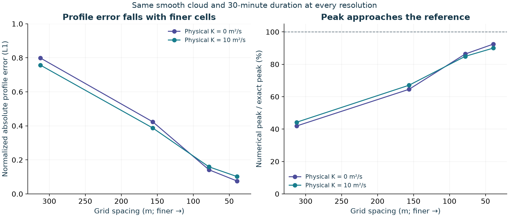
| 64 | 312.5 | 30.000 | 0.7576 | 44.2% | 333.75 |
| 128 | 156.25 | 30.000 | 0.3876 | 67.1% | 99.37 |
| 256 | 78.125 | 19.191 | 0.1591 | 84.9% | 30.98 |
| 512 | 39.0625 | 8.897 | 0.1018 | 90.0% | 18.60 |
“Normalized profile error” is the sum of absolute differences in cell masses divided by initial mass. It is a whole-profile diagnostic, not percentage error at a home, and is not a health metric. Peak comparison uses exact and numerical cell averages at each matching resolution. Extra numerical mixing is inferred from the excess variance growth; it is not a measured atmospheric diffusivity.
With K = 0, baseline peak/reference ratios rise from 41.9% at 312.5 m spacing to 92.5% at 39.0625 m. Profile error decreases at every spatial refinement in both K cases. Error reduction is not a constant factor because the stability-limited time step and Courant number also change. Only four finite resolutions were tested; this does not establish convergence of the terrain application.
Why shortening the time step did not fix it
For this first-order upwind method, reducing the time step at fixed grid spacing increases numerical spreading. At 312.5 m spacing with K = 10, the inferred extra mixing rises from approximately 333.75 to 401.25 to 435.00 m²/s as the step is reduced from 30 to 15 to 7.5 seconds. The chosen physical mixing remains 10 m²/s. This behaviour follows the scheme's discrete variance equation; it does not justify choosing a time step to obtain a preferred map.
For uniform positive wind u, spacing Δx, physical mixing K and elapsed time T, the interior update predicts:
variance(T) − variance(0) = 2 K T + u Δx T − u² Σ(Δt²)
The sum uses every actual step, including the shortened final step. Mean and variance are calculated from cell-integrated masses at cell centres. The exact reference uses the same cell-centre weighting; we do not mistake that discrete representation for the continuum variance. Gaussian integrals use Python's standard-library complementary error function to retain small tails.
Checks, including the failures
304 of 312 predeclared computational checks pass; 8 fail. All 28 runs conserve the tracked mass budget, remain finite and nonnegative, require no negative-mass clipping, and preserve the crosswind/vertical uniform profile within the specified tolerances. The largest relative mass-budget residual is 6.45e-15.
The eight failed checks are four strict centroid checks and four strict variance-equation checks in the coarse 20 km domain with half/quarter time steps. The thresholds were 0.00001 m for centroid and 0.01 m² for variance. Tiny escaping tails bias these sensitive whole-cloud moments: the largest lost fraction is 1.35e-08 (about 0.014 parts per million of initial tracer mass). The maximum centroid discrepancy is about 0.00012 m and the maximum variance discrepancy about 1.052 m². The failed flags and nonzero verification exit status remain in the download.
All four extended-domain controls pass the moment checks, and their interior profiles differ from the matched original-domain profiles by at most 6.04e-11 of initial mass. The quarter-step controls directly test the largest failures. No additional extended-domain half-step browser-engine run was made; the separate Python replay also checked that half-step boundary explanation. These controls support lost-tail bias as the explanation and show that boundaries do not account for the large profile/peak error. They do not erase the original failed checks.
Reproduction and review status
The download includes frozen inputs and protocol, exact engine, a Node runner, Python Gaussian-reference generator, full results, CSV metrics, figures and their plotting script. It also includes a separate AI-assisted protocol review and independent Python replay. The replay compares a separately written one-dimensional update and reference calculations with the browser output; it is an internal computational cross-check, not independent human scientific review.
Run node run.cjs inside the unzipped folder. With the frozen experiment it is expected to exit with status 1 because the eight recorded moment checks fail. Inspect results.json for each result. Do not change those thresholds to turn the status green. Standard-library Python supports the separate replay and reference generation; recreating figures additionally requires Matplotlib. File hashes identify the archived inputs and outputs, not scientific approval.
What remains unresolved
This test excludes terrain flow, changing winds, inversions, buoyant flare rise, chemical conversion, actual emissions and ambient background. It neither replaces nor clears the earlier failed 48-to-64-column real-terrain refinement. It does not estimate ground-level exposure at a home, health risk, or a safe distance. Successful arithmetic and decreasing error in this smooth case cannot supply those missing validations.
For scientific review, the immediate questions are whether the custom map calculation should remain an educational illustration, what suitable dispersion pathway should support future quantitative mapping, and which current source and local weather records would make that assessment reproducible. See the review guide and prioritized data requests.